Introduction to Neural Networks for Advanced Deep Learning(Part 2).

It is very easy for humans to understand the image of a cat below but how can a computer do it?

Neural networks are at the core of modern deep learning, driving advancements across various fields such as computer vision, natural language processing, and robotics. In this second blog post, we will provide a comprehensive introduction to neural networks, covering key concepts that everyone needs to understand when dealing with this powerful class of models.

The human visual ability is very impressive, it is effortless to determine the image above but our brain contains millions of neurons and billions of interconnection that makes it very easy to know. What if we need a computer to know that this is the cat?

A computer program can be written to understand the patterns in the image this works with some of the mathematics behind it. We will use this example to know how can computer neurons learn this image and understand whether it is a cat image or any other. Let us see how this works.

To make a computer understand an image, we need to convert it into a specific format using pixels. In this example, the image of a handwritten digit 8 needs to be turned into a readable format of 28 x 28 pixels. This means the computer would process the image as 28 x 28 = 784 inputs to understand it properly.

Consider the calculations and demonstration made below, in any image to insert it into the network as input it has to be readable as input numbers. we take an image as pixels for 28 x 28 we will have 784 inputs that will be inserted into neurons.

Each neuron in a neural network is connected to others and multiplied by their weights. These weights are numbers between 0 and 1, they determine how much importance should be given to specific image pixels. Weights are important in neural networks, they can reduce or enhance the importance of input data.

In simple terms, when weight has a large value, it means the feature has more trust compared to other features. The weighted sum of inputs is then added to a numerical value called BIAS. Next, the input goes through an activation function in the hidden layers, where most of the processing happens. The activation function acts as a threshold, and the processed input is then passed to the next layer.

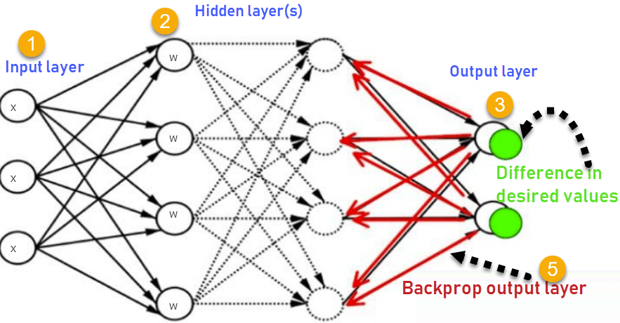
After processing, the final output is a probability number. If the output is correct, that's great. However, if the network makes mistakes, it determines the difference between the output value and the real value used during training. To correct these mistakes, a process called backpropagation takes place. The error calculated during backpropagation determines the changes needed to reduce the error.

The information is sent backward through the network, that is, backpropagated. This process continues until the weights can predict the true values accurately. It might take some time for this learning process to converge and make accurate predictions.

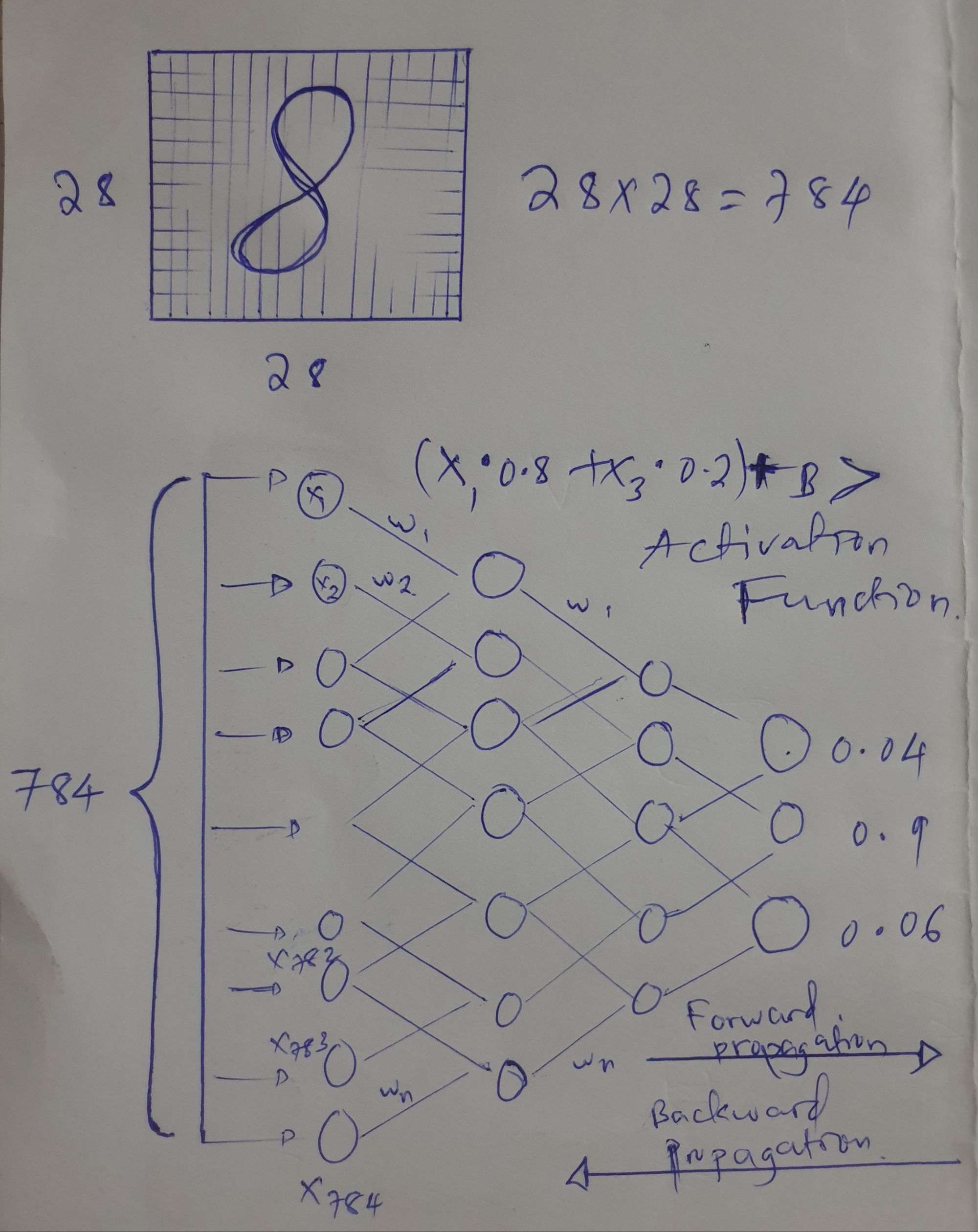
In the picture above, there's an image written digit 8 it has made of 28 x 28 tiny dots (pixels), which gives 784 inputs for the neurons. Then, we follow the steps explained above as well. The information moves forward through the neural network (forward propagation). After all the calculations are done, the image is checked and corrected for any errors using backward propagation until we finally get the correct name or result.

Do not be tired, we have a general concept so let us summarize our time by explaining those common terms mentioned above.

1. Neurons and Activation Functions.

At the heart of a neural network are artificial neurons, inspired by the functioning of biological neurons in the human brain. Each neuron receives input from multiple sources, applies a weighted sum to these inputs, and then passes the result through an activation function this activation function acts as a threshold point to get the final probability of our number in the end. This process is very important crucial for the network to learn complex patterns in data.

Common activation functions include:

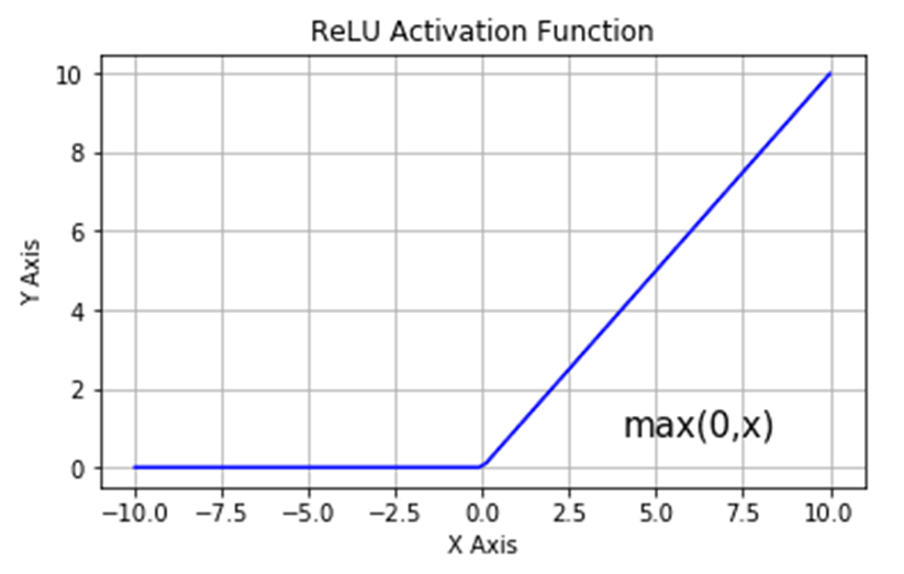
• ReLU (Rectified Linear Unit): f(x) = max(0, x). It is widely used due to its simplicity and ability to mitigate the vanishing gradient problem.

• Sigmoid: f(x) = 1 / (1 + exp(-x)). It maps inputs to a range between 0 and 1, making it suitable for binary classification tasks.
• TanH (Hyperbolic Tangent): f(x) = (2 / (1 + exp(-2x))) - 1. Similar to the sigmoid function, but it maps inputs to a range between -1 and 1.

To have an in-depth understanding of these functions read HERE or WATCH

2. Layers and Architecture

Neural networks consist of layers, which contain a set of neurons. The three main types of layers are:

• Input Layer: Receives the data as input. The number of neurons in this layer corresponds to the dimensions of the input data.
• Hidden Layer: Intermediate layers between the input and output layers. They help the network learn complex representations from the input data.
• Output Layer: Produces the final output of the neural network. The number of neurons in this layer depends on the nature of the task (e.g., binary classification, multi-class classification, regression).

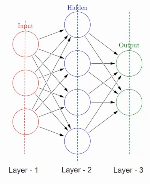
The architecture of a neural network refers to its specific arrangement of layers, including the number of neurons in each layer and the connections between them.

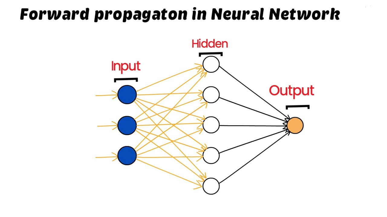
3. Forward Propagation

Forward propagation is the process by which input data is inserted through the neural network, and predictions are generated. During this process, the input travels through each layer, and the activations are done using the weighted sum of inputs and activation functions.

Mathematically, forward propagation can be summarized as follows:

1. Initialize the input with the data given.
2. Calculate the weighted sum of the input for each neuron in a layer.
3. Apply the activation function to obtain the output of each neuron.
4. Pass the outputs to the next layer as inputs, and repeat the process until reaching the final output layer.

4. Loss Function

The loss function measures the difference between the predicted output and the actual target. It finds the model's performance and acts as the feedback signal for learning. The goal of training a neural network is to minimize the loss function and improve the accuracy of predictions.

Common loss functions may include:

• Mean Squared Error (MSE): Suitable for regression tasks.

5. Backpropagation

Backpropagation is also used to train neural networks. It involves calculating the loss function with respect to the  (weights and biases) and then adjusting these parameters using optimization algorithms like Gradient Descent or its variants.

The process of backpropagation can be summarized as follows:

1. Perform forward propagation to make predictions and find the loss.
2. Calculate the gradients of the loss function with respect to each parameter using the chain rule of calculus( let us skip this calculus for now)
3. Update the parameters using an optimization algorithm to minimize the loss.

6. Optimization Algorithms

Optimization algorithms are used to find the optimal set of weights and biases that minimize the loss function. Some optimization algorithms include:

• Gradient Descent: The basic algorithm for updating parameters based on the gradient of the loss function.
• Adam ( Adaptive Moment Estimation ): This is also an algorithm for optimization techniques for gradient descent. The method is efficient when working with large problems involving a lot of data or parameters. It requires less memory and is efficient

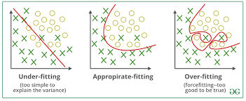
7. Overfitting and Regularization

Overfitting is a common issue in neural networks where the model performs well on the training data but poorly on unseen data. Regularization techniques are employed to avoid overfitting. Some regularization techniques include L1 and L2 regularization, dropout, and batch normalization.

Conclusion

To this end, we look an introduction to neural networks for advanced deep learning in its core terms. We look at important concepts like neurons, activation functions, layers, forward propagation, loss functions, backpropagation, optimization algorithms, and regularization.

Let me give you BYE BYE until the next blog!.

Let's keep the chat: Mgasa Lucas

Recommended reference:  WATCH

Happy learning!